Week 10-11: Detailed Benchmarking Analysis
Follow on from the Last Post
In the last blog post, I discussed the creation of a test system to evaluate the performance improvement of streaming the WESTPA trajectories. In that post I was using the chignolin protein as a test system. Using this system as a benchmark, I found that there was no significant performance improvement from analysing on-the-fly versus analysing after the simulation was finished. To diagnose the lack of improvement, I timed the analysis script in order to identify whether any speed up would be expected from the streaming approach. Timing the analysis script revealed that the script only takes 3.3 seconds to run. This explains why no speed up was seen from the streaming approach as this time is insignificant compared to the simulation time. Even though in this analysis we are calculating a number of pairwise distances, the small size of the chignolin protein means that the computational cost of the analysis is low and no speed up is seen. To see a speed up from the streaming approach, we need to use a system where the analysis takes a significant amount of time.
Theoretical Analysis of Speed Up
To understand the potential speed up from the streaming approach, we can perform a theoretical analysis. The total time taken for one WESTPA iteration can be approximately expressed as (ignoring overhead from starting and ending the iteration itself):
\begin{equation} \tau_{iteration} = \frac{N_{segments}}{N_{sims}} \cdot \tau_{segment} \label{eq:iteration_time} \end{equation}
Where \(N_{segments}\) is the number of segments in the iteration, \(N_{sims}\) is the number of simulations that can be run in parallel and \(\tau_{segment}\) is the time taken for one segment. Without streaming, the time taken for one segment can be approximated as a sum of the simulation time and the analysis time:
\begin{equation} \tau_{segment - no streaming} = \tau_{sim} + \tau_{analysis} \label{eq:segment_time_no_streaming} \end{equation}
Combining equation \ref{eq:iteration_time} and \ref{eq:segment_time_no_streaming} leads to an expression for the total iteration time without streaming:
\begin{equation} \tau_{iteration - no streaming} = \frac{N_{segments}}{N_{ sims}} \cdot (\tau_{sim} + \tau_{analysis}) \label{eq:iteration_time_no_streaming} \end{equation}
For the streaming approach, the analysis is performed on-the-fly during the simulation. In this case, a simple model can approximate the time taken for one segment as the maximum of the simulation time and the analysis time:
\begin{equation} \tau_{segment - streaming} = \max(\tau_{sim}, \tau_{analysis}) \label{eq:segment_time_streaming} \end{equation}
However, this assumes that the analysis and the simulation can be performed in perfect parallel. In reality, the analysis will always only be able to end after the simulation has ended as the final frame has to be analysed. We can adjust equation \ref{eq:segment_time_streaming} to account for this by adding a small overhead term \(\tau_{analysis-singleframe}\) which accounts for the time taken to analyse the final frame: \begin{equation} \tau_{segment - streaming} = \max(\tau_{sim} + \tau_{analysis-singleframe}, \tau_{analysis}) \label{eq:segment_time_streaming_adjusted} \end{equation}
Combining equation \ref{eq:iteration_time} and \ref{eq:segment_time_streaming_adjusted} leads to an expression for the total iteration time with streaming: \begin{equation} \tau_{iteration - streaming} = \frac{N_{segments}}{N_{s ims}} \cdot \max(\tau_{sim} + \tau_{analysis-singleframe}, \tau_{analysis}) \label{eq:iteration_time_streaming} \end{equation} From equations \ref{eq:iteration_time_no_streaming} and \ref{eq:iteration_time_streaming}, we can derive an expression for the theoretical speed up, \(S\), from using the streaming approach: \begin{equation} S = \frac{\tau_{iteration - no streaming}}{\tau_{iteration - streaming}} = \frac{\tau_{sim} + \tau_{analysis}}{\max(\tau_{sim} + \tau_{analysis-singleframe}, \tau_{analysis})} \label{eq:speed_up} \end{equation} Writing in terms of the ratio of analysis time to simulation time \(\alpha = \frac{\tau_{analysis}}{\tau_{sim}}\) and assuming that \(\tau_{analysis-singleframe}\) is negligible, we can get a very simple expression for \(S\): \begin{equation} S = \frac{1 + \alpha}{\max(1, \alpha)} \label{eq:speed_up_simple} \end{equation}
This function is plotted below:
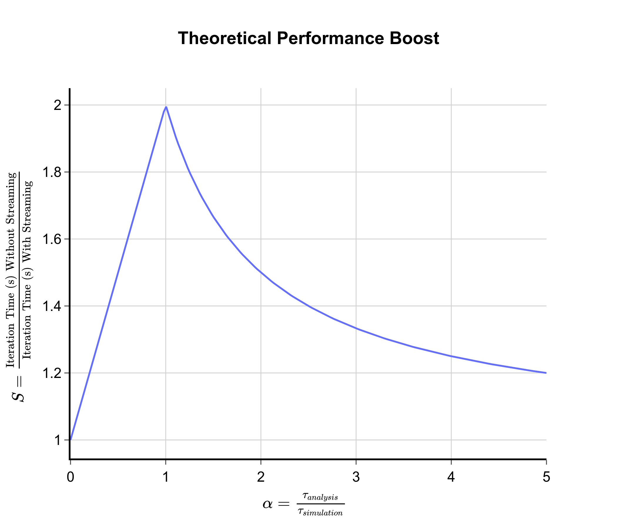
From this graph, we can see that peak speed up occurs when \(\alpha = 1\), i.e. when \(\tau_{analysis} \approx \tau_{sim}\). This corresponds to a factor of 2 speed up. When \(\tau_{analysis} \ll \tau_{sim}\), \(\alpha \approx 0\) and there is no speed up from the streaming approach as the analysis time is negligible compared to the simulation time. This was the case with the chignolin test system. When \(\tau_{analysis} \gg \tau_{sim}\), \(\alpha \gg 1\) and there is again little speed up from the streaming approach. This is because the analysis time is so long that performing it on-the-fly does not significantly reduce the total time taken. In this case, it would be better to optimise the analysis code to reduce \(\tau_{analysis}\). From this analysis, we can conclude that to see a significant speed up from the streaming approach, we need to use a test system where the analysis time is approximately equal to the simulation time.
The Collagen Fibril as a New Test System
To achieve a better balance between analysis time and simulation time and to explore the potential benefits of the streaming approach, I decided to use a collagen fibril model as a new test system. I chose this system as I have spent many years of my PhD studying collagen and so I had the simulation files already set up! In the collagen molecule, there are around 3000 protein residues in total making it significantly larger than the chignolin protein. Similar to the chignolin test system, I am calculating a number of pairwise distances between residues. However, due to the larger size of the collagen molecule, the number of pairwise distances is much larger leading to a longer analysis time. Due to wanting quick benchmarking and availability of resources, I used a segment time of only 2 ps with only 5 cores per segment. This leads to a single simulation taking around 1 minute. By adjusting the frequency at which the system is analysed (i.e. analysing every 10 steps vs every 100 steps), we can modify the ratio of the analysis time to the simulation time and get real estimates for the speed up. The actual performance gain as a function of alpha from using the streaming approach is shown in the graph below:
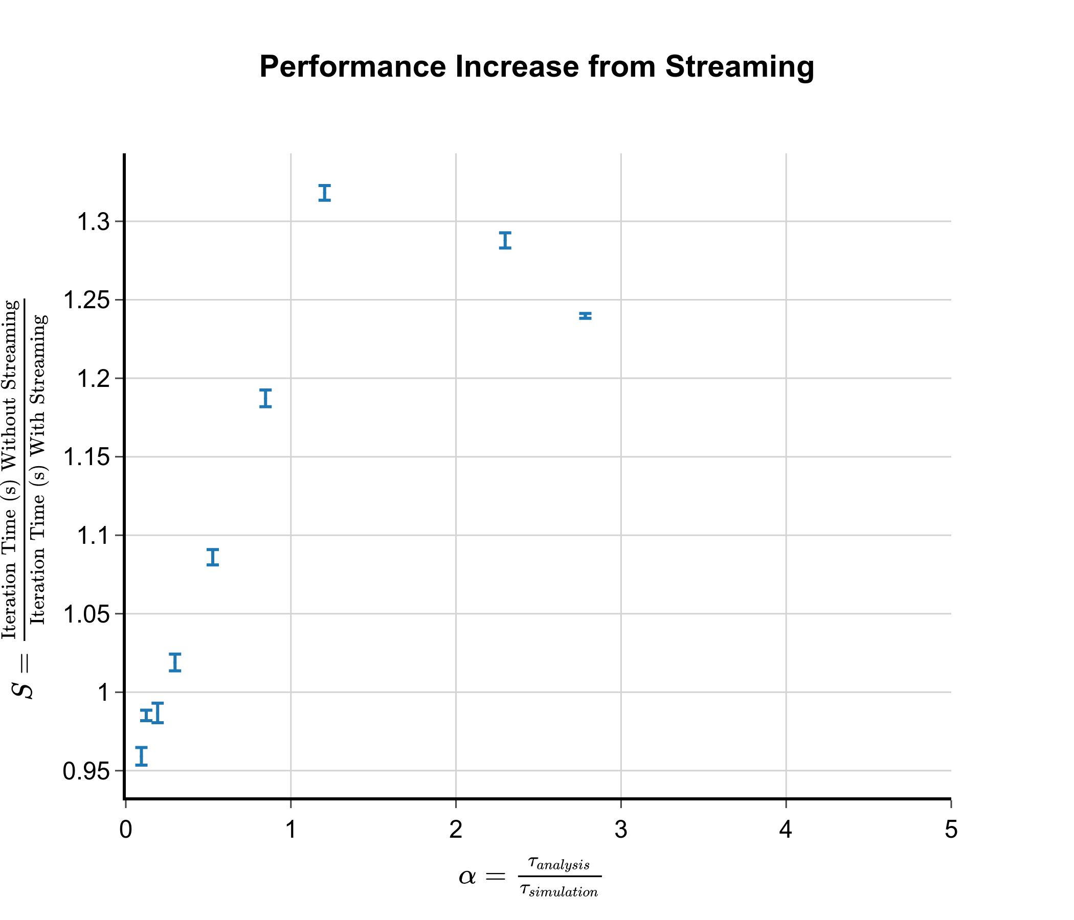 As can be seen from the graph, the realised performance boost closely follows the theoretical predictions, with peak speed up occurring at the same point where \(\alpha = 1\). The max performance boost we obtain is only 1.3 times compared to the theoretical value of 2.0. This is because some part of the iteration will have to be performed in serial and there will be some overhead caused by setting up the streaming. Another important graph is the plot of iteration time against number of analysed points. This gives us an idea of how much the streaming approach unlocks the possibility of more complicated analyses.
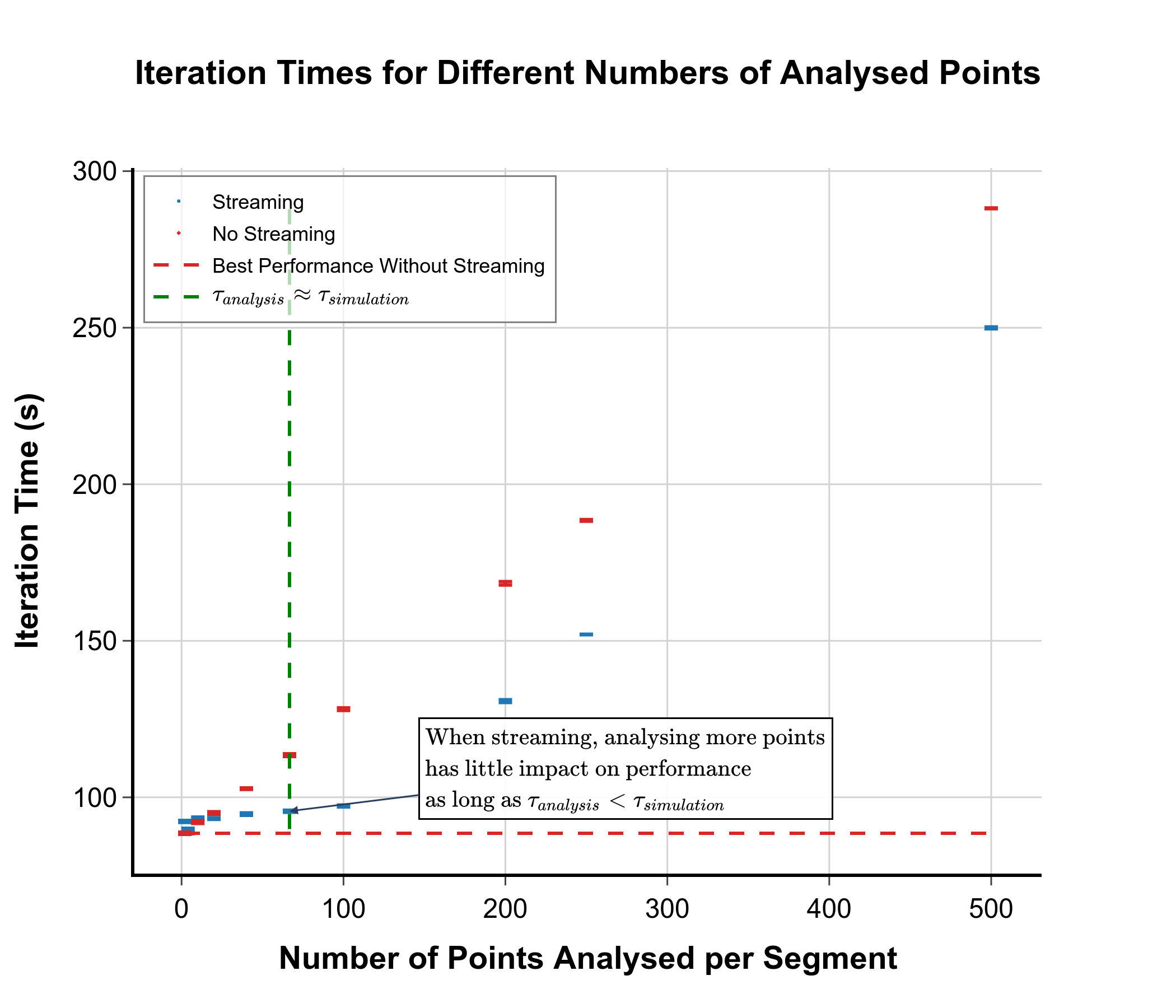 As can be seen from the graph, as long as the time to analyse a segment is less than the time taken to simulate the segment, it is relatively “free” to increase the complexity of the analysis or to increase the number of analysed points. This means that we can perform more analyses as the simulation is running without incurring significant additional costs, potentially reducing the amount of data that has to be stored.
When is Streaming Useful?
The analysis above gives us some simple rules for when streaming is likely to be beneficial. I recommend the user measures the time it takes for a single segment to be simulated and measures the time it takes to perform the desired analysis on the data for that segment. If the analysis time is comparable to or shorter than the simulation time, then streaming is likely to provide a speed up. In addition, the user can increase the number of analysed points for very little cost as long as the analysis time remains shorter than the simulation time.